Evidence Review

Prevention Services Clearinghouse ratings are applied to contrasts. A contrast is defined as a comparison of a treated condition to a counterfactual condition on a specific outcome. For example, a study with one intervention group and one comparison group that reports findings on one outcome has a single contrast. A study with one intervention group and one comparison group that reports findings on two outcomes would have two contrasts, one for each of the comparisons between the intervention and comparison group on the two outcomes. Contrasts will be reviewed from randomized controlled trial or quasi-experimental designs.

Most studies report results on more than one outcome and some studies have more than two conditions (e.g., more than one treated condition and/or more than one comparison condition). When studies report results on more than one outcome or compare two or more different intervention groups to a comparison group, the study is reporting results for multiple contrasts. Prevention Services Clearinghouse ratings can differ across the contrasts reported in a study; that is, a single study may have multiple design and execution ratings corresponding to each of its reported contrasts.

The design and execution ratings from multiple contrasts and (if available) multiple studies are used to determine the program or service rating. Program or service ratings are described in Chapter 6. The current chapter is focused on the procedures for rating a contrast against the design and execution standards.

For each contrast in an eligible study, Prevention Services Clearinghouse reviewers determine a separate design and execution rating. This assessment results in any of the following ratings, shown in order from strongest to weakest evidence:

• Meets Prevention Services Clearinghouse Standards for High Support of Causal Evidence
• Meets Prevention Services Clearinghouse Standards for Moderate Support of Causal Evidence
• Meets Prevention Services Clearinghouse Standards for Low Support of Causal Evidence

Because the level of evidence can differ among multiple contrasts reported in a study, Prevention Services Clearinghouse reviewers apply design and execution ratings to each contrast separately. Thus, a single study that reports multiple contrasts might be assigned multiple different design and execution ratings. For example, a quasi-experimental design study may report impact estimates for two outcome measures, one of which has a pre-test version of the outcome that satisfies requirements for baseline equivalence, the other of which does not satisfy baseline equivalence requirements. The first contrast may receive a moderate rating while the second would receive a low rating.

Exhibit 5.1 presents a summary of the designs that are eligible to receive high and moderate ratings. Details regarding how these ratings are derived are provided in the sections that follow.

Exhibit 5.1. Summary of Designs Eligible to Meet Design and Execution Standards

Meets Prevention Services Clearinghouse Standards for High Support of Causal Evidence	Meets Prevention Services Clearinghouse Standards for Moderate Support of Causal Evidence
Randomized studies that meet: Standards for integrity of random assignment (Section 5.4) Standards for low risk of joiner bias (Section 5.5) Attrition standards (Section 5.6) Baseline equivalence standards for randomized studies (Sections 5.7 and 5.8) Statistical model standards (Section 5.9.1) All measurement standards (Section 5.9.2) All design confound standards (Section 5.9.3) Missing data standards (Section 5.9.4)	Randomized studies that fail standards for integrity of random assignment (Section 5.4) or attrition (Section 5.6) and quasi-experimental studies that meet: Baseline equivalence standards (Sections 5.7 and 5.8) Statistical model standards (Section 5.9.1) All measurement standards (Section 5.9.2) All design confound standards (Section 5.9.3) Missing data standards (Section 5.9.4)
Meets Prevention Services Clearinghouse Standards for Low Support of Causal Evidence
Contrasts that are reviewed and fail to meet high or moderate standards

The Review Process Differs for RCTs versus QEDs

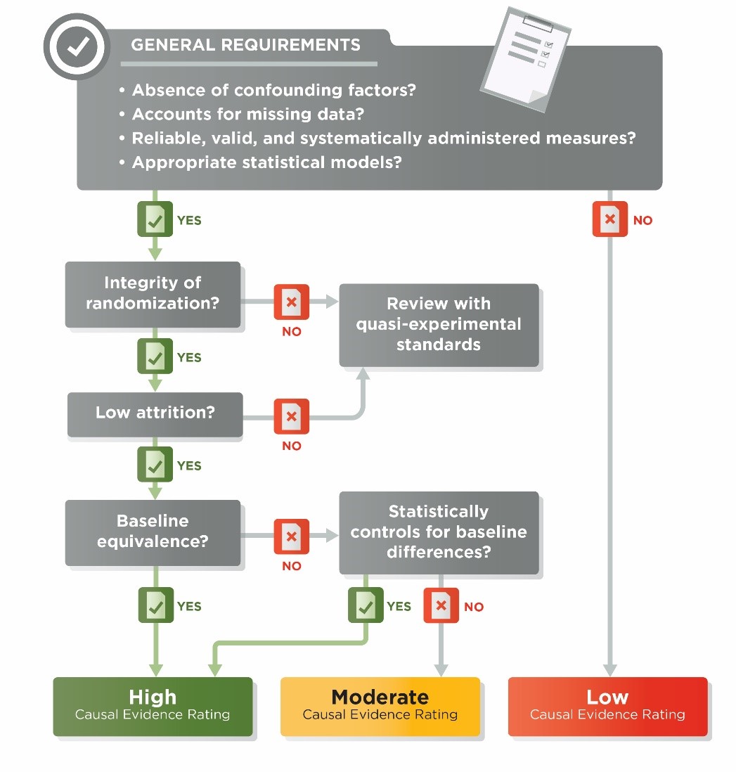
When Prevention Services Clearinghouse reviewers rate the evidence produced from a study contrast, they begin by making a determination about whether random assignment was used to create the contrast. Once that determination is made, they follow the sequence of steps in the flow charts depicted in Exhibit 5.2 for RCTs and Exhibit 5.5 for QEDs. The various decisions and standards that apply are described in the accompanying text.

The first step in the review process involves determining whether a contrast was created using a randomized controlled trial (RCT) design or a quasi-experimental design (QED). To be reviewed as a randomized controlled trial, the unit of assignment may be either individuals or groups of individuals (i.e., clusters), but the individuals or clusters must be assigned using a random process and each individual or cluster must have a nonzero probability of being assigned to either condition. The probability of assignment to conditions can differ across individuals or clusters (e.g., it is acceptable for a study to assign 60% of the participants to an intervention group and 40% of the participants to a comparison group).

• If assignment to conditions is based on a random process, reviewers first assess the integrity of the randomization and attrition (see Sections 5.4 through 5.6).
• If a contrast does not use random assignment, reviewers follow the steps for QEDs that begin with an assessment of baseline equivalence (see Section 5.7).

For RCTs, reviewers evaluate the integrity of the random assignment process. The integrity of random assignment is evaluated for both individual and cluster assignment RCTs. Contrasts in which the initial random assignment to intervention or comparison conditions was subsequently compromised fail the criterion for integrity of random assignment. These contrasts may be reviewed by the Prevention Services Clearinghouse as quasi-experimental designs. The following examples illustrate ways in which random assignment can be compromised.

5.4.1 Examples of Compromised Random Assignment of Individuals

Example 1: In a study where initial assignment to intervention and comparison groups was made by a random process, the researcher identifies individuals who were randomly assigned to the intervention group, but who refused to participate in the intervention. The researcher either reclassifies those individuals as belonging to the comparison group or drops those individuals from the analysis sample. In this example, the randomization has been undermined and the study would not be classified as a study using random assignment of individuals.

Exhibit 5.2. Ratings Flowchart for Contrasts from Randomized Controlled Trials

Example 2: In a multi-site study, individuals are randomly assigned to intervention and comparison groups within 20 sites. One of the sites would not allow randomization, so assignment to intervention and comparison groups was done by a method other than randomization. Data from all 20 sites are included in the analysis. The site with the non-random assignment has undermined the random assignment for the whole study, and the multi-site study would not be classified as a study using random assignment of individuals.

Example 3: In a study where initial assignment to intervention and comparison groups was made by a random process, the service provider is concerned because many of the individuals who were assigned to the intervention group are refusing treatment. To fill the empty treatment slots, the service provider identifies additional individuals who meet the study eligibility criteria and assigns them to the intervention group to ensure a full sample of participants. The analysis includes individuals originally assigned to the intervention group via randomization and the additional intervention members added later. In this example, the randomization has been undermined and the study would not be classified as a study using random assignment of individuals.

Example 4: In a study where initial assignment to intervention and comparison groups was made by a random process, the service provider is concerned because many of the individuals who were assigned to the intervention group are refusing treatment. To fill the empty treatment slots, the service provider recruits some of the comparison group members to participate in treatment. In the analysis, the researcher includes those treated comparison group members as belonging to the intervention group. In this example, the randomization has been undermined and the study would not be classified as a study using random assignment of individuals.

5.4.2 Examples of Changes to Random Assignment That Are Acceptable

Example 5: In a study where the initial assignment to intervention and comparison groups was made by a random process, the service provider is concerned because many of the individuals who were assigned to the intervention group are refusing treatment. To fill the empty treatment slots, the service provider recruits some individuals who were not assigned to either the intervention or comparison group in the original randomization to fill the empty slots. In the analysis, the researcher maintains the original treatment assignments, and excludes the subsequently recruited individuals from the impact analyses. In this example, the randomization has not been undermined and the study would be classified as a study using random assignment of individuals.

Example 6: Randomization to intervention and comparison groups was conducted within blocks or pairs but all intervention group members or all comparison group members of the pair or block have attrited (no outcome data are available for those members). The integrity of the randomization is not compromised if the entire pair or block is omitted from the impact analysis. For example, groups of three similar clinics were put into randomization blocks; within each block, two clinics were randomized to the intervention condition and one to the comparison condition. During the study, a clinic closes in one of the blocks, and no outcome data were able to be collected from that clinic. The researcher dropped all three members of the block from the analysis. In this example, randomization has not been compromised.

If a contrast was created by randomly assigning clusters to conditions and the randomization has not been compromised, reviewers then evaluate the potential for risk of bias from individuals joining the sample after the randomization occurred. Only cluster randomizations are evaluated for joiner bias.

A contrast is created by random assignment of clusters if groups of individuals (e.g., entire communities, clinics, families) are randomly assigned to intervention and control conditions, and all individuals that belong to a cluster are assigned to the intervention status of that cluster.

Cluster randomized contrasts may be subject to risk of bias if individuals can join clusters after the point when they could have known the intervention assignment status of the cluster. The risk exists if individuals can be placed into clusters after the point when the person making the placement knows the intervention assignment status of the clusters.

In such cases, individuals with different characteristics or motivations may be more likely to self-select or be assigned to one condition. When individuals can self-select into or are placed into clusters after the clusters’ intervention status is known, any observed difference between the outcomes of intervention and comparison group members could be due not only to the intervention’s impact on individuals’ outcomes in the cluster, but also to the intervention’s impact on the composition of the clusters (i.e., the intervention’s impact on who joined or was placed into the clusters).
The Prevention Services Clearinghouse design and execution rating standards are focused on assessing the impacts of interventions on the outcomes of individuals. Therefore, if the observed impact of the intervention could be partially due to changes in the composition of clusters (for example, if individuals who are prone to more favorable outcomes are more likely to join or be placed in intervention clusters), then the impact on the composition of the clusters has biased the desired estimate of the intervention’s impact on individuals’ outcomes.

A cluster randomized contrast has a low risk of joiner bias in two scenarios. The first is if all individuals in a cluster joined or were placed in the cluster prior to the point when they could have plausibly known the intervention assignment status of the cluster. The second is if individuals are placed into clusters before the point when the person making the placement knows the intervention assignment status of clusters.

A cluster randomized contrast could also have low risk of joiner bias if it is very unlikely that knowledge of the intervention status would have influenced the decision to join the cluster. This holds whether individuals could join clusters soon after randomization (early joiners), or even long after randomization (late joiners).
Some contrasts may be created by randomly assigning families to conditions and then evaluating program impacts on multiple parents/caregivers and/or multiple children within those families. The Prevention Services Clearinghouse considers contrasts created this way to be cluster RCTs. Generally, reviewers assume that cluster RCTs in which families are assigned to conditions have low risk of joiner bias. That is, parents/caregivers and/or children who join families during a study are not considered to bias the impact estimates.

Contrasts created by randomly assigning clusters other than families (e.g., clinics, communities) are assumed to have low risk of joiner bias only if they have no joiners (i.e., all individuals were cluster members before knowledge of the intervention assignment status of the clusters). The exceptions to the “only if they have no joiners” requirement may include situations where the availability of the intervention isn’t publicized or isn’t noticeable to likely participants or where transfer from one provider to another is not common or allowed.

The Prevention Services Clearinghouse assumes that there is high risk of joiner bias whenever individuals are placed into clusters after the person making the placement knows the intervention assignment status of clusters. For example, if mental health clinics in a network are randomly assigned to intervention and comparison conditions, and the network administrator places families in clinics after knowing which clinics are in the intervention condition, then the Prevention Services Clearinghouse assumes that there is high risk of joiner bias.

• If reviewers determine that there are no individuals in the sample who joined clusters after assignment or there is low risk for joiner bias, they then assess attrition (see Section 5.6).
• If reviewers determine that there is high risk of joiner bias due to individuals joining clusters after assignment, attrition is not assessed and they move directly to examining baseline equivalence (see Section 5.7).

In RCTs, individuals or clusters that leave the study sample can reduce the credibility of the evidence. When the characteristics of the individuals or clusters who leave are related to the outcomes, this can result in groups that are systematically different from each other and bias the estimate of the impact of an intervention. Therefore, if a contrast is constructed using individual random assignment or is determined to be cluster randomized with no joiners or low risk of joiner bias, reviewers evaluate attrition.

Because both overall attrition from a sample and differential attrition from intervention and comparison conditions can compromise the integrity of randomization, reviewers evaluate both overall and differential attrition. Attrition is evaluated differently for individual and cluster randomized studies, as described in the subsections below.

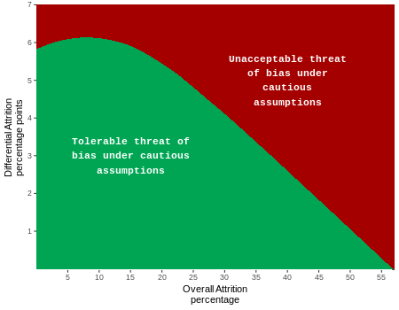
The Prevention Services Clearinghouse bases its standards for attrition on those developed by the What Works Clearinghouse (WWC), which applies “optimistic” boundaries for attrition for use with studies where it is less likely that attrition is related to the outcomes, and “cautious” boundaries for use with studies where there is reason to believe that attrition may be more strongly related to the outcomes. The WWC’s attrition model is based on assumptions about potential bias as a function of overall and differential attrition. The Prevention Services Clearinghouse uses the cautious boundary for all studies. This reflects the presumption that attrition in studies with the high risk populations of interest to the Prevention Services Clearinghouse may be linked with the outcomes targeted in Clearinghouse reviews. For example, if families at greater risk of entry into the child welfare system are more likely to drop out of a study, this can bias the results; this bias can be even more problematic if there is differential dropout between intervention and comparison groups. Exhibit 5.3 illustrates the combinations of overall and differential attrition that result in tolerable and unacceptable bias using the cautious boundary. Exhibit 5.4 shows the numeric values for the Prevention Services Clearinghouse attrition boundaries.

Exhibit 5.3. Potential Bias Associated with Overall and Differential Attrition

Overall Attrition	Differential Attrition		Overall Attrition	Differential Attrition		Overall Attrition	Differential Attrition
0	5.7		20	5.4		40	2.6
1	5.8		21	5.3		41	2.5
2	5.9		22	5.2		42	2.3
3	5.9		23	5.1		43	2.1
4	6.0		24	4.9		44	2.0
5	6.1		25	4.8		45	1.8
6	6.2		26	4.7		46	1.6
7	6.3		27	4.5		47	1.5
8	6.3		28	4.4		48	1.3
9	6.3		29	4.3		49	1.2
10	6.3		30	4.1		50	1.0
11	6.2		31	4.0		51	0.9
12	6.2		32	3.8		52	0.7
13	6.1		33	3.6		53	0.6
14	6.0		34	3.5		54	0.4
15	5.9		35	3.3		55	0.3
16	5.9		36	3.2		56	0.2
17	5.8		37	3.1		57	0.0
18	5.7		38	2.9
19	5.5		39	2.8

Source: What Works Clearinghouse (n.d.)
Note: Overall attrition rates are given as percentages. Differential attrition rates are given as percentage points.

5.6.1 Attrition in Studies with Random Assignment of Individuals

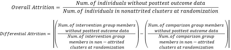
In contrasts with individual random assignment, overall attrition is defined as the number of individuals without post-test outcome data as a percentage of the total number of members in the sample at the time that they learned the condition to which they were randomly assigned, specifically:

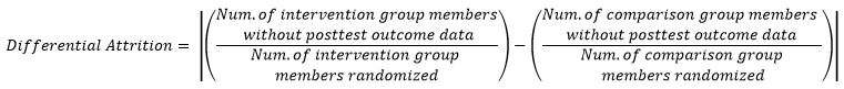
Differential attrition is defined as the absolute value of the percentage point difference between the attrition rates for the intervention group and the comparison group, specifically:

The timing of randomization is central to the calculation of attrition for the Prevention Services Clearinghouse. For the purposes of defining the sample for the attrition calculation, randomization of individuals to conditions is considered to have occurred once individuals learn their assignment condition. This moment is defined as the earliest point in time at which any of the following occur:

• Individuals are explicitly informed about the condition to which they were assigned, or
• Individuals begin to experience the condition to which they were assigned, or
• Individuals could have plausibly deduced or have been affected by assignment to their condition, or
• Individuals have not yet experienced any of the conditions above, but their counterpartshave experienced it.

When eligibility and consent (if needed) is determined prior to the point in time when individuals learn their assignment condition, the Prevention Services Clearinghouse defines attrition of an individual as an individual who learned their assignment condition, but for whom an outcome measurement was not obtained. In this scenario, ineligible and unconsented individuals are not counted in the attrition calculation. This definition reflects an understanding that if an individual did not know, or could not have plausibly known their intervention status before withdrawing from a study, then the intervention assignment could not have affected a decision to participate in the study or not. If consent is obtained after the point that individuals know their assignment condition, and no outcome measures are obtained on unconsented individuals, then the unconsented individuals are counted as attrition.

Occasionally, studies apply exclusionary conditions after the point when individuals learn their assignment condition. For the Prevention Services Clearinghouse, if the study used the same exclusionary conditions in both the intervention and the comparison groups, then eligibility criteria can be applied after that time point and ineligible individuals can be excluded from the attrition calculations and from the analysis.

Example 1: A mental health prevention program is targeted to children at risk for behavior problems. A researcher receives nominations from parents and teachers for 100 children, who are then randomly assigned to conditions. All children in both conditions are then given a diagnostic screening. Those scoring above a criterion on the screener are defined as ineligible and are excluded from the study sample. Because the same exclusion was applied in exactly the same way in both conditions, the excluded children do not need to be counted for the purpose of the attrition calculation.

Example 2: In the same study as in Example 1, a therapist in the intervention condition recognizes that one of her participants does not meet the diagnostic criteria. On her recommendation, the child transfers out of the program. For the purposes of the attrition calculation, this child must be included in the sample and cannot be classified as ineligible, because no similar screen was applied in the comparison group and a similar child who had been randomized to the comparison group would not have been identified and removed. If the researchers continue to identify the child as belonging to the intervention group for the purposes of their impact analysis, and they obtain an outcome measurement for the child, no attrition has occurred. If no outcome measurement is obtained on this child, then attrition has occurred.

Example 3: For a clinic-based study, researchers create a randomized ordering of intervention and comparison assignments and save the list to a secure website. When individual “A” walks into a clinic, an employee of the clinic does an eligibility screen. Individual “A” is determined to be eligible, and the clinic employee successfully recruits the individual to participate in the study. Individual “A” is then asked to complete a baseline survey, which she does. The clinic employee then goes to the secure website and finds the next unused randomization status record and finds that the assignment is to the intervention group. The employee tells the participant her randomization status, at which point she learns that she was randomized to receive services. Although she refuses services, an outcome measure is obtained for her, and the researcher maintains her assignment status as “intervention group” in the analysis and uses her outcome measure in the analysis. (In this example, the researcher utilizes an intent-to-treat analysis because individuals are analyzed as members of the condition to which they were originally assigned). Individual “A” has not attrited from the study.

Example 4: In the same study as Example 3, individual “B” walks into the clinic and is determined to be eligible, and the clinic employee successfully recruits the individual to participate in the study. Individual “B” is then asked to complete a baseline survey, but does not complete it and says she wants to withdraw from the study. Individual “B” has not attrited from the study because neither she nor the clinic employee knew her randomization status at the time of her withdrawal.

Example 5: In the same study as Examples 3 and 4, individual “C” is determined to be eligible, and the clinic employee successfully recruits the individual to participate in the study. Individual “C” completes her baseline survey and learns her assignment condition. No outcome measurement is obtained for individual “C.” Individual “C” has attrited from the study.

5.6.2 Attrition in Studies with Random Assignment of Clusters

In contrasts with randomization of clusters, if the contrasts exhibit low risk of joiner bias or no individuals join the sample, reviewers assess overall and differential attrition at both the cluster and individual levels. In cluster randomized contrasts, individual-level attrition is calculated only in non-attrited clusters. An attrited cluster is one in which no outcome measures were obtained for any members of the cluster. For cluster studies, individual-level overall and differential attrition are calculated as:

• For cluster randomized contrasts that are deemed to have high risk of joiner bias, attrition is not relevant to the review and the contrasts are required to demonstrate baseline equivalence (see Section 5.7).
• For each contrast in a study for which attrition must be assessed, reviewers determine both overall and differential attrition at the individual level and, if applicable, at the cluster level. If attrition is determined to be below the boundaries shown in Exhibit 5.3, the contrast is said to have low attrition. If attrition is above the boundary, the contrast is said to have high attrition. Baseline equivalence is evaluated for both low and high attrition RCTs, as well as for all QEDs, using the standards described next (see Section 5.7).

All contrasts from studies that receive full reviews by the Prevention Services Clearinghouse are assessed for baseline equivalence. In some cases, when estimating impacts, contrasts must control for the variables that are out of balance at baseline (see Section 5.7.3). Although the baseline equivalence assessment is applied to all contrasts, the assessment can affect the ratings for those created from RCTs and QEDs differently. The ratings flowchart for RCTs shown in Exhibit 5.2 illustrates how the baseline equivalence standard is applied to RCTs. The ratings flowchart for QEDs shown in Exhibit 5.5 illustrates how the baseline equivalence standard is applied to QEDs.

The Prevention Services Clearinghouse thresholds for baseline equivalence are based on those used by the WWC. Specifically, baseline equivalence is assessed by examining baseline differences expressed in effect size (ES) units. Baseline effect sizes less than 0.05 are considered equivalent and no further covariate adjustments are required. Baseline effect sizes between 0.05 and 0.25 indicate that statistical adjustments in the impact models may be required (see Section 5.8); these baseline effect sizes are said to be in the adjustment range. Baseline effect sizes greater than 0.25 are addressed differently for low attrition RCTs versus all other designs. When statistical adjustments are required, the Prevention Services Clearinghouse standards for acceptable adjustment models described in Section 5.8 below are applied.

An exact match between the analytic sample size used to assess baseline equivalence and the analytic sample size used to estimate an impact is preferred for demonstrating baseline equivalence. Whenever there is less than an exact match in sample size between the analytic sample used to assess baseline equivalence and the sample used to estimate an impact, the Prevention Services Clearinghouse applies the WWC v4.0 standards for estimating the largest baseline difference (see Section 5.9.4). If the largest baseline difference is less than 0.25 standard deviation units, the contrast can receive a moderate rating.

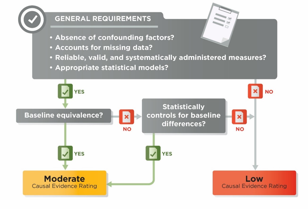
Exhibit 5.5. Ratings Flowchart for Quasi-experimental Design Studies

5.7.1 Conducting the Baseline Equivalence Assessment

When assessing baseline equivalence, reviewers first determine whether there is a direct pre-test on the outcome variable. In general terms, a pre-test is a pre-intervention measure of the outcome. More specifically, a measure satisfies requirements for being a pre-test if it uses the same or nearly the same measurement instrument as is used for the outcome (i.e., is a direct pre-test), and is measured before the beginning of the intervention, or within a short period after the beginning of the intervention in which little or no effect of the intervention on the pre-test would expected. If there is a direct pre-test available, then that is the variable on which baseline equivalence must be demonstrated.

For some outcomes, a direct pre-test either is impossible (e.g., if the outcome is mortality), or not feasible (e.g., an executive function outcome for 3-year-olds may not be feasible to administer as a pre-test with younger children). In such cases, reviewers have two options for conducting the baseline equivalence assessment. These options are only permitted for contrasts for which it was impossible or infeasible to collect direct pre-test measures on the outcomes.

1. Pre-test alternative. A pre-test alternative is defined as a measure in the same or similar domain as the outcome. These are generally correlated with the outcome, and/or may be common precursors to the outcome. When multiple acceptable pre-test alternatives are available, reviewers select the variable that is most conceptually related to the outcome prior to computing the baseline effect size. The selection of the most appropriate pre-test alternative is documented in the review and confirmed with Prevention Services Clearinghouse leadership.
2. Race/ethnicity and socioeconomic status (SES). If a suitable pre-test alternative is not available, baseline equivalence must be established on both race/ethnicity and SES.
   • Race/ethnicity. For baseline equivalence on race/ethnicity, reviewers may use the race/ethnicity of either the parents or children in the study. When race/ethnicity is available for both parents and children, reviewers select the race/ethnicity of the individuals who are the primary target of the intervention. In some studies, the race/ethnicity groupings commonly used in the U.S. may not apply (e.g., studies conducted outside the U.S.). In such cases, reviewers perform the baseline equivalence assessment on variables that are appropriate to the particular cultural or national context in the study.
   • Socioeconomic Status (SES). For baseline equivalence on SES, the Prevention Services Clearinghouse prefers income, earnings, federal poverty level in the U.S., or national poverty level in international contexts. If a preferred measure of SES is not available, the Prevention Services Clearinghouse accepts measures of means-tested public assistance (such as AFDC/TANF or food stamps/SNAP receipt), maternal education, employment of a member of the household, child or family Free and Reduced Price Meal Program status, or other similar measures.

In addition, reviewers examine balance on race/ethnicity, SES, and child age, when available, for all contrasts, even those with available pretests or pretest alternatives. If any such characteristics exhibit large imbalances between intervention and comparison groups, Prevention Services Clearinghouse leadership may determine that baseline equivalence is not established. Evidence of large differences (ES > 0.25) in demographic or socioeconomic characteristics can be evidence that the individuals in the intervention and comparison conditions were drawn from very different settings and are not sufficiently comparable for the review. Such cases may be considered to have substantially different characteristics confounds (see Section 5.9.3).

Reviewers examine the following demographic characteristics, when available:

• Socioeconomic status. Socioeconomic status may be measured with any of the following: income, earnings, federal (or national) poverty levels, means-tested public assistance (such as AFDC/TANF or food stamps/SNAP receipt), maternal education, employment of a member of the household and child, or family Free and Reduced Price Meal Program status.
• Race/ethnicity. Reviewers may assess child or parent/caregiver race/ethnicity, depending on what data are available in a study.
• Age. For studies of programs for children and youth, reviewers will assess baseline equivalence on child/youth age.

5.7.2 Other Baseline Equivalence Requirements

Variables that exhibit no variability in a study sample cannot be used to establish baseline equivalence. For example, if a study sample consists entirely of youth with a previous arrest, a binary indicator of that variable cannot be used to establish baseline equivalence because there is no variability on that variable.

5.7.3 How the Baseline Equivalence Assessment Affects Evidence Ratings

Randomized Studies with Low Attrition

For RCTs with low attrition, reviewers examine baseline equivalence on direct pre-tests, or pre-test alternatives or race/ethnicity and SES. If the baseline effect sizes are <0.05 standard deviation units, the contrast can receive a high rating. If the baseline effect sizes are > 0.05 standard deviation units, the contrast can receive a high rating only if the baseline variables are controlled in the impact analyses (see Section 5.8). If baseline effect sizes cannot be computed, but impact analyses clearly include the baseline variables that are required, the contrast can receive a high rating. If the baseline effect sizes are >.05 or appropriate baseline variables are not available and statistical controls are not used, the contrast can receive a moderate rating, provided other design and execution standards are met.

Randomized Studies with High Attrition and Quasi-Experimental Design Studies

For RCTs with high attrition and for all QEDs, reviewers examine baseline equivalence on direct pre-tests, or pre-test alternatives or race/ethnicity and SES. If the baseline effect sizes are <0.05 standard deviation units, the contrast can receive a moderate rating. If the baseline effect sizes are between 0.05 and 0.25 standard deviation units, the contrast can receive a moderate rating only if the baseline variables are controlled in the impact analyses (see Section 5.8). If statistical controls are not used, the contrast receives a low rating. If direct pre-tests are not possible or feasible and no pre-test alternatives or race/ethnicity and SES are available, baseline equivalence is not established for the outcome and that contrast receives a low rating.

When the baseline equivalence assessment determines that an impact model must control for a baseline variable in order to meet evidence standards, any of the following approaches for statistical control are acceptable:

• Regression models with the baseline variables as covariates. This includes all commonly understood forms of regression including ordinary least squares, multi-level or generalized linear models, logistic regression, probit, and analysis of covariance.
• Gain score models where the dependent variable in the regression is a difference score equal to the outcome minus the pre-test.
• Repeated measures analysis of variance models.
• Difference-in-difference models (these must use pre-tests, not other baseline variables).
• Models with fixed effects for individuals (these must use pre-tests, not other baseline variables).

All RCTs and QEDs that meet the requirements described above for attrition and baseline equivalence, and use acceptable methods for pre-test controls that are appropriate for the respective design and circumstances must also meet additional requirements to receive a rating of high or moderate. These requirements address issues related to the statistical models used to estimate program impacts, features of the measures and measurement procedures used in the studies, confounding factors, and missing data.

5.9.1 Statistical Model Standards

The Prevention Services Clearinghouse design and execution ratings apply standards for the statistical models that are used to estimate impacts. The statistical model standards include the following:

• When there is unequal allocation to intervention and comparison conditions within randomization blocks the impact model must account for the unequal allocation using any of the three approaches listed below. If impact models do not appropriately account for the unequal allocation, reviewers follow the steps for quasi-experimental designs.
  • Use dummy variables in the impact model to represent the randomization blocks
  • Reweight the observations such that weighted data have equal allocations to intervention and control within each randomization block
  • Conduct separated impact analyses within each block and average the impacts across the blocks.
• Impact models cannot include endogenous measures as covariates. If the impact model for a contrast includes endogenous covariates and alternate model specifications (without such covariates) or unadjusted means and standard deviations on the outcome variable are not available, the contrast receives a low rating.
  • An endogenous covariate is one that is measured or obtained after baseline and that could have been influenced by the intervention. Inclusion of endogenous covariates results in biased impact estimates.
• The Prevention Services Clearinghouse may, in some cases, determine that a statistical model is invalid for estimating program impacts such as when data are highly skewed or if there are obvious collinearities that make estimates of program impacts suspect or uninterpretable.

5.9.2 Measurement Standards

Prevention Services Clearinghouse standards for outcomes, pre-tests, and pre-test alternatives apply to all eligible outcomes and are aligned with those in use by the WWC. Specifically, there are three outcome standards: face validity, reliability, and consistency of measurement between intervention and comparison groups.

Face Validity

To satisfy the criterion for face validity, there must be a sufficient description of the outcome, pre-test, or pre-test alternative measure for the reviewer to determine that the measure is clearly defined, has a direct interpretation, and measures the construct it was designed to measure.

Reliability

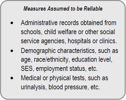
Reliability standards apply to all outcome measures and any measure that is used to assess baseline equivalence. They are not applied to other measures that may be used in impact analyses as control covariates. To satisfy the reliability standards, the outcome or pre-test measure either must be a measure which is assumed to be reliable (see the box on the right) or must meet one or more of the following standards for reliability:

• Internal consistency (such as Cronbach’s alpha) of 0.50 or higher.
• Test-retest reliability of 0.40 or higher.
• Inter-rater reliability (percentage agreement, correlation, or kappa) of 0.50 or higher.

When required, reliability statistics on the sample of participants in the study under review are preferred, but statistics from test manuals or studies of the psychometric properties of the measures are permitted.

Consistency of Measurement between Intervention and Comparison Groups

The Prevention Services Clearinghouse standard for consistency of measurement requires that:

• Measures are constructed the same way for both intervention and comparison groups.
• The data collectors and data collection modes for data collected from intervention and comparison groups either are the same or are different in ways that would not be expected to have an effect on the measures.
• The time between pre-test (baseline) and post-test (outcome) does not systematically differ between intervention and comparison groups.

Prevention Services Clearinghouse reviewers assume that measures are collected consistently unless there is evidence to the contrary.

Example 1: In a study of a teen pregnancy prevention program, intervention group participants are asked about sexual behavior outcomes in a face-to-face interview with a case worker. Comparison group participants are asked in an online survey. In this example, the study would fail to meet Prevention Services Clearinghouse standards for consistency of measurement.

Example 2: In a mental health program, an anxiety assessment is distributed to youth by an interventionist and collected from the interventionists after the allotted time expires. In the comparison condition, community center staff distribute and collect the assessment using the same procedures. In both conditions, the same anxiety assessment is used and the test forms are sent to the researcher, who scores the results. Although different types of staff distributed and collected the assessment, this would not be expected to affect the test results. In this example, the outcome would not fail to meet Prevention Services Clearinghouse standards for consistency of measurement.

• outcome measures must meet all of the measurement standards for a contrast to receive a moderate or high rating.
• pre-tests or pre-test alternatives that do not meet the measurement standards cannot be used to establish baseline equivalence.

5.9.3 Design Confound Standards

The strength of causal inferences can be affected by the presence of confounding factors. A confounding factor is present if there is any factor, other than the intervention, that is both plausibly related to the outcome measures and also completely or largely aligned with either the intervention group or the comparison group. In such cases, the confounding factor may have a separate effect on the outcome that cannot be eliminated by the study design or isolated from the treatment effect. In such cases, it is impossible to separate how much of the observed effect was related to the intervention and how much to the confounding factor. Thus, the contrast cannot meet evidence standards and will receive a low rating. In QEDs, confounding is almost always a potential issue because study participants are not randomly assigned to intervention and comparison groups and some unobserved factors may be contributing to the outcome. Statistical controls cannot save contrasts from the effect of a confound if one is present.

The Prevention Services Clearinghouse defines two types of confounds: the substantially different characteristics confound, and the n=1 person-provider or administrative unit confound.

Substantially Different Characteristics Confound

Even when intervention and comparison groups are shown to meet standards for equivalence at baseline, or when baseline differences between intervention and comparison groups are adjusted for in analytic models, the effect of an intervention on outcomes can be sometimes be confounded with a characteristic of the treated or comparison units, or with a characteristic of the service providers, especially if that characteristic differs systematically between intervention and comparison groups. The characteristic that differs between the two groups may be related to the expected amount of change between pre-test and post-test measurements, thus confounding the intervention effect.

Prevention Services Clearinghouse defines a “substantially different characteristics confound” to be present if a characteristic of one condition, or a characteristic of the service provider for one condition, is systematically different from that of the other condition. For example, a substantially different characteristics confound may exist if there are large demographic differences between the groups, even if the groups are equivalent on the pre-test. In the case of a systematic difference between a service provider characteristic, the characteristic is not a confound if the characteristic is defined to be a component or requirement of the intervention.

One standard that is applied in Prevention Services Clearinghouse reviews is “refusal of offer of treatment.” When the intervention group comprises individuals or units that were offered and accepted treatment and most or all of the comparison group comprises individuals or units that were known to have been offered and refused treatment, Prevention Services Clearinghouse defines the design to have a substantially different characteristics confound. The Prevention Services Clearinghouse assumes that refusal or willingness to participate in treatment is likely to be related to motivation or need for services, which are likely to be related to outcomes.

Many QED studies will have intervention groups that consist entirely of individuals or units that accepted the offer of treatment. In these circumstances, the strongest designs would limit the comparison group members to those that would have been likely to accept the treatment if offered. The Prevention Services Clearinghouse, however, does not currently differentiate evidence ratings for studies that do and do not limit the comparison group in this manner. Some comparison groups will include individuals for whom it is unknown whether they would have participated in treatment had it been offered. The Prevention Services Clearinghouse does not consider this scenario to have a substantially different characteristics confound.

Example 1: A mental health intervention is targeted to families at risk of entry into the child welfare system, and is offered to families who have had at least one unsubstantiated claim of abuse or neglect in the past year. The comparison group consists of at risk families who have been nominated by school social workers in the same community but who have not had any claims of abuse or neglect. A substantially different characteristics confound is present because families in the intervention group have a characteristic that is substantially different from the comparison group that is plausibly related to outcomes.

n=1 Person-Provider Confound or Administrative Unit Confound

When all individuals in the intervention group or all individuals in the comparison group receive intervention or comparison services from a single provider (e.g., a single therapist or a single doctor) the treatment effect is confounded with the skills of the provider. For example, when intervention services are provided by a single therapist and the pre-post gains of her patients on a mental health assessment are compared with the gains of patients of another therapist, it is impossible to disentangle the effect of the intervention from the skills of the therapists. The Prevention Services Clearinghouse calls this type of confound an n=1 person provider confound because only one individual person is providing services, and it is impossible to disentangle the provider effects from the treatment effect.

Similar to the n=1 person-provider confound, when all individuals in the intervention group or all individuals in the comparison group receive intervention or comparison services in a single administrative unit (e.g., clinic, community, hospital) the treatment effect may be confounded with the capacity of that administrative unit to produce better outcomes. The Prevention Services Clearinghouse calls this type of confound an n=1 administrative unit provider confound.

5.9.4 Missing Data Standards

The Prevention Services Clearinghouse uses the WWC v4.0 standards for missing data with the exception that that the standards are applied only to post-tests on eligible outcome measures, pre-tests, and pre-test alternatives. For other model covariates, any method that is used to address missing data is acceptable.
If a contrast has missing data on post-tests, pre-tests, or pre-test alternatives, reviewers first assess whether the approach to addressing missing data is one of the acceptable approaches described below.

• If a contrast has missing data and does not use one of the acceptable approaches listed below, it receives a rating of low.
• If a contrast has missing data and an acceptable method for addressing the missing data is used, reviewers then proceed based on whether the contrast was created via randomization or not.

The following approaches are acceptable for addressing missing data:

• Complete Case Analysis: Also known as listwise deletion. Refers to the exclusion of observations with missing data from the analysis. For RCTs, cases excluded due to missing data are counted as attrition. For QEDs, if baseline equivalence is established on the exact analytic sample as the impact analyses, there are no further missing data requirements. If the sample for baseline equivalence is not identical to the sample used in the impact analyses, additional requirements to assess potential bias due to missing data apply, as described below.
• Regression Imputation. Regression-based single or multiple imputation conducted separately for intervention or comparison groups (or that includes an indicator variable for intervention status) in which all covariates in the imputation are included in the impact models and that includes the outcome in the imputation.
• Maximum Likelihood: Model parameters are estimated using an iterative routine. Standard statistical packages must be used.
• Non-Response Weights: Weighting based on estimated probabilities of having missing outcome data. Acceptable only for missing post-tests and if the weights are estimated separately for intervention and comparison groups or if an indicator for intervention group status is included.
• Constant Replacement: Replacing missing values with a constant value and including an indicator variable in impact estimation models to identify the missing cases. Acceptable only for RCTs with missing pre-tests and pre-test alternatives.

Procedures for Low Attrition RCTs with Missing Data

If a contrast was created from randomization of individuals or clusters, reviewers assess attrition; imputed outcomes are counted as attrition. That is, reviewers count cases with missing outcomes as if they had attrited.

If attrition is low, the contrast can receive an evidence rating of high, provided that all other design and execution standards are met, and an acceptable method of addressing missing data is used. When attrition is low and an acceptable method of addressing missing data is used, impact estimates from models with imputed missing data are acceptable for computing effect sizes and statistical significance.

Procedures for High Attrition RCTs and Quasi-Experiments with Missing Data

If a contrast from a RCT exhibits high attrition (with any imputed cases counted as attrition) or was not created by randomization (i.e., is a QED), reviewers must assess whether the contrast limits the potential bias that may result from using imputed outcome data. If no outcome data are imputed, potential bias from imputed outcome data is not present.

If outcome data are imputed, reviewers calculate an estimate of the potential bias from using imputed outcome data and assess whether that estimate is less than 0.05 standard deviation units of the outcome measure. To estimate the potential bias, reviewers use a pattern-mixture modelling approach, as outlined in Andridge and Little (2011; see also the What Works Clearinghouse Standards, v4.0) and operationalized in a spreadsheet-based tool (Price, 2018).

• If the potential bias is greater than the 0.05 threshold, the contrast receives a low rating.
• If the potential bias is less than the 0.05 standard deviation unit criterion and the contrast is a high attrition RCT that analyzes the full randomized sample using imputed data, then the contrast can receive a moderate evidence rating, provided other design and execution standards are met and an acceptable method of addressing missing data is used.
• If the potential bias is less than the 0.05 standard deviation threshold but the full randomized sample is not used or the contrast is a QED and no pre-test or pre-test alternatives are imputed, reviewers evaluate baseline equivalence for the analytic sample and proceed as usual for contrasts required to establish baseline equivalence.

If pre-test or pre-test alternative data are imputed or the full analytic sample is not available for baseline equivalence, additional computations to determine the largest baseline difference are applied (Andridge & Little, 2011; What Works Clearinghouse Standards, v4.0). These computations are operationalized in a spreadsheet tool (Price, 2018).

• If the contrast fails to satisfy the largest baseline difference criterion, it receives a low rating.
• If criterion contrast satisfies the largest baseline difference criterion, it may receive an evidence rating of moderate, provided the other design and execution standards are met and an acceptable method of addressing missing data is used.

All contrasts in a study are rated against the design and execution standards regardless of the magnitude or statistical significance of the impact estimate. For any contrast that receives a high or moderate design and execution rating, reviewers record or compute an effect size in the form of Hedges’ g, its sampling variance (or standard error), and statistical significance, correcting as necessary for clustering. If data are not available for such computations, reviewers may send queries to authors requesting such information, in accordance with the author query policies described in Section 7.3.2. If requested data are not obtained in response to author queries, reviewers complete the review with the information available. The Prevention Services Clearinghouse must be able to determine if impact estimates are statistically significant for them to be used to inform program ratings.

In addition, the Prevention Services Clearinghouse applies the following procedures to all effect size computations:

• Because errors and omissions in reporting p-values and statistical significance are common, the Prevention Services Clearinghouse computes the statistical significance for all contrasts, and does not rely on reporting by study authors (Bakker & Wicherts, 2011; Krawczyk, 2015).
• Only aggregate findings are recorded and rated under this Version 1.0 of the Prevention Services Clearinghouse. Future versions of the Handbook may address subgroup findings.
• Impact estimates that are favorable (statistically significant and in the desired direction), unfavorable (statistically significant and not in the desired direction), or sustained favorable (statistically significant and in the desired direction at least 6 or 12 months beyond the end of treatment, see Section 6.2.3) are used to determine program or service ratings, but all impacts from all contrasts rated as high or moderate are recorded.

5.10.1 Procedures for Computing Effect Sizes

The Prevention Services Clearinghouse uses the standardized mean difference effect size metric for outcomes measured on a continuous scale (e.g., group differences in average scores on an assessment of mental health). All effect sizes are recorded or computed such that larger effect sizes represent positive outcomes for the intervention condition. The basic formulation of the standardized mean difference effect size (d) is

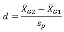
where the numerator is the difference in group means for the intervention and comparison groups, and the denominator is the pooled standard deviation of the intervention and comparison groups. All standardized mean difference effect sizes are adjusted with the small-sample correction factor to provide unbiased estimates of the effect size (Hedges, 1981). This small-sample corrected effect size (Hedges’ g) can be represented as:

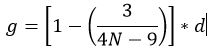
and the sampling variance of the effect size is represented as

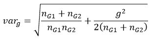
where N is the total sample size for the intervention and comparison groups, g is the effect size, nG1 is the sample size for the intervention group, and nG2 is the sample size for the comparison group.

For binary outcomes, the Prevention Services Clearinghouse computes effect sizes as odds ratios and then converts them to standardized mean difference effect sizes using the Cox transformation as described in Sánchez-Meca, Marín-Martínez, and Chacón-Moscoso (2003).
Standard formulae for computing effect sizes from common statistical tests are employed, as necessary (Lipsey & Wilson, 2001).

5.10.2 Adjusting for Pre-Tests

Reviewers use statistics that are adjusted for pre-tests and other covariates to compute effect sizes whenever possible. In cases where statistical adjustments are not required (i.e., low attrition RCTs or studies with baseline effect sizes <0.05) and study authors report only unadjusted pre-test and post-test findings, reviewers compute the effect size of the difference between the intervention and comparison groups at baseline and subtract that value from the post-test effect size.

5.10.3 Procedures for Correcting for Mismatched Analysis

In the event that studies reviewed by the Prevention Services Clearinghouse report findings for clustered data that have not been appropriately corrected for clustering, reviewers apply a clustering correction to the findings. The Prevention Services Clearinghouse applies this correction to findings from mismatched analyses; that is, analysis for which the unit of assignment and unit of analysis are mismatched and not appropriately analyzed using, for example, multi-level models. The intraclass correlations required for this adjustment is taken from the studies under review when possible. When intraclass correlations are not available, a default value of .10 is used, consistent with the conventions used by the What Works Clearinghouse for non-academic measures.

5.10.4 Reporting and Characterizing the Effect Sizes on the Prevention Services Clearinghouse Website

The individual findings from each contrast with a high or moderate rating are reported on the Prevention Services Clearinghouse website. These findings include the effect size, its statistical significance, and a translation of the effect size into percentile units called the implied percentile effect. In addition, meta-analysis is used to summarize the findings for each outcome domain. The Prevention Services Clearinghouse uses a fixed effect weighted meta-analysis model using inverse-variance weights (Hedges & Vevea, 1998) to estimate the average effect size for each domain.

Prevention Services Clearinghouse reviewers also convert each effect size into percentile units for reporting on the Prevention Services Clearinghouse website to provide a user-friendly alternative to the effect sizes. This implied percentile effect is the average intervention group percentile rank for the outcome minus the comparison group average percentile, which is 50. For example, an implied percentile effect of 4 means that the program or service increased the intervention group performance by 4 percentile points over the comparison group.